Basic statistics for quality of service assessment
06.06.2020Means
Quality of service measurements are typically concerned with numbers like:
- The proportion of call set-ups that are successful.
- The mean of the times taken by file downloads.
To provide the numbers, “events” (such as call set-ups and file downloads) are observed. The “observations” are numerical values of important facts about the events. For instance, in these examples they could be:
- 1 for a successful call set-up and 0 for an unsuccessful call set-up.
- The time taken by a file download.
In this note observations are also called “measurements” and are used to calculate “measurement results.”
Perhaps the commonest measurement result found in everyday life is the “mean.” This is the sum of the observations divided by the total number of observations. It is what is usually, but not always, called the “average.”
The proportion of events that have some property is the mean of observations which count 1 for an event that has the property and 0 for any other event. For instance, observations of whether call set-ups are successful and of whether file downloads take at most 30 seconds determine:
- The proportion of call set-ups that are successful.
- The proportion of file downloads that take at most 30 seconds.
- There are means which are not proportions because they deal with the natures of events not the numbers of events. In particular, observations of times taken to download files determine:
- The mean of the times taken by file downloads.
As some attempts to download files might fail or take too long to be observed in realistic practice, there could also be interest in, for example:
- The mean of the times taken by file downloads that take at most 30 seconds.
Standard deviations
A further important measurement result is the “variance,” which indicates the amount of variation in the observations. It is the average of the squares of the differences between the observations and their mean. Commonly the “standard deviation,” which is the square root of the variance, appears instead of the variance in equations and is used to indicate how far the observations deviate from the mean.
Quantiles
There is much to be said for just considering means, which are relatively well understood, especially when presenting quality of service information to customers. However, in some cases there are other informative measurement results, such as:
- The maximum of the times taken by the fastest 80 per cent of file downloads.
This time is an 80 per cent “quantile” (or “80th percentile”), which is taken in this note to be the largest among the smallest 80 per cent of the observations when they are arranged in increasing order. It might be useful if, for example, many events take times with almost the same length as each other but important exceptions take very long times.
The 50 per cent quantile is the “median.” It is the largest among the smallest 50 per cent of the observations when they are arranged in increasing order, if there is an odd number of observations; it is the mean of that value and the next value higher in the order, if there is an even number of observations. It is sometimes what is meant by the “average.”
Yet another possible “average” is the “mode,” which is the most popular value among the observations, if that value is unique.
Confidence intervals and credibility intervals
Looking at samples of events, instead of all events, can reduce the cost and complexity of making observations. The measurement results for samples of events are then estimates of those for all events together. For instance, the mean of observations on a sample of events, which is a measurement result, is an estimate of the mean of observations on all of the events in the population from which the sample comes. In this note the mean of observations on all of the events is called the “true value.” The pattern of the events together is a “distribution.”
If the sample size is large enough, a measurement result for the sample can be a good enough estimate of the true value. Often “being a good enough estimate” means “having a big enough chance that the measurement result for the sample is within a little enough distance of the true value;” then the “little enough distance” is called the “confidence interval” or the “credibility [credible] interval” (CI) and the “big enough chance” is called the “confidence level” or the “credibility [credible] level” (CL).
The “big enough chance” that is wanted can vary between applications, but for many years it has usually been taken to be 19 out of 20, or 95 per cent, in which case there is said to be a “95 per cent CL” and a “little enough distance” is a “95 per cent CI.” A “90 per cent CL” and a “90 per cent CI” are also sometimes used, in which case the chance is 9 out of 10, or 90 per cent.
For instance, if the mean of the times taken by sample file downloads is 25 seconds, there might need to be a 95 per cent CL that the interval between 24 seconds and 26 seconds encompasses the true value. This CL would be justified only if the sample size was large enough. However, the sample size should not be so large that observations are economically or technically infeasible.
The abbreviation “CI” (with “CL”) is used in this note to mask the distinction between confidence intervals (and levels) and credibility intervals (and levels). In fact:
- A 95 per cent confidence level indicates how frequently something should happen: the 95 per cent confidence interval constructed around a measurement result encompasses the true value for 95 per cent of the measurement results.
- A 95 per cent credibility level indicates how definitely something has happened: the 95 per cent credibility interval constructed around a measurement result is 95 per cent likely to encompass the true value.
This distinction stems from differences in the meaning and calculation of probabilities. Arguably confidence intervals are less appropriate than credibility intervals to quality of service monitoring, because field tests are not repeated in fully comparable circumstances. However, confidence intervals are less difficult to calculate than credibility intervals in general. In this article, attention is limited to cases where confidence intervals and credibility intervals overlap so much for large enough sample sizes that the differences between them are imperceptible in quality of service monitoring; the formulae mentioned relate to confidence intervals, but the quantities provided relate equally well to credibility intervals.
The CL indicates how well the measurement results for samples act as estimates of true values for the populations from which the samples come. It thereby indicates the statistical significance of the results. However, the results might have statistical significance without having practical significance. For instance, the mean of the times taken by file downloads in a sample might be 25 seconds, in which case if the sample size was large enough there might be a 95 per cent CL that the true value was between 23 seconds and 27 seconds; the closeness to the true value would have statistical significance, but it would not have practical significance unless users could detect it. Only when measurement results have practical significance do sample sizes need to be large enough to ensure statistical significance.
Sample sizes for calculating estimates of means
Making observations sometimes entails measuring times to answer such questions as:
- “How long does it take to set up calls?”
- “How long does it take to resolve complaints?”
- “How long does it take to transmit messages?”
- “How long does it take to look up addresses?”
- “How long does it take to download files?”
- “How long does it take to repair faults?”
The most useful measurement result is frequently the mean of the observations, giving, for example:
- The mean of the times taken to set up calls.
- The mean of the times taken to resolve complaints.
- The mean of the times taken to transmit messages.
- The mean of the times taken to look up addresses.
- The mean of the times taken to download files.
- The mean of the times taken to repair faults.
When observations are used to estimate a mean, an important fact (known as the “central limit theorem”) can help to ensure that sample sizes are large enough. It states that, as the sample sizes grow, the distribution of the means of the observations comes to resemble a so-called “normal” or Gaussian distribution, so a sample that is large enough for estimating means in the normal distribution will be large enough for estimating means in other distributions. This is so for all possible observations (provided that they are independent, identically distributed, and come from a distribution with a finite standard deviation).
For a CI around the mean for a sample coming from the normal distribution, a large enough sample size is (z*z)*(s*s)/(d*d) (with rounding upwards). Here:
- d is half the length of the CI (and, for a CI symmetric about the mean, is the absolute difference between the mean and the minimum or maximum value in the CI).
- s is the standard deviation of the observations (or, in other words, an indication of how far the observations deviate from the mean).
- z determines the chance that the CI encompasses the true value (and is about 1.96 for a 95 per cent CL or 1.65 for a 90 per cent CL).
For instance, if, for a sample of file downloads the mean of the times is 25 seconds and the standard deviation of the times is 10 seconds (as might happen if the downloads take between 5 seconds and 45 seconds on 95 per cent of occasions) then, for the file downloads in the population from which the sample comes:
- There is a 95 per cent CL that the mean of the times is between 23 (=25-2) seconds and 27 (=25+2) seconds, provided that there are at least (1.96*1.96)*(10*10)/(2*2), or about 96, files in the sample.
- There is a 95 per cent CL that the mean of the times is between 24 (=25-1) seconds and 26 (=25+1) seconds, provided that there are at least (1.96*1.96)*(10*10)/(1*1), or about 384, files in the sample.
Thus, ensuring that a sample size is large enough entails not only estimating the mean of what is being measured but also finding information about the standard deviation.
When observations are used to estimate a quantile, a fact similar to the central limit theorem can help to ensure that sample sizes are large enough: again, as the sample sizes increase, the distribution of the means of the observations comes to resemble a normal distribution. In this case, however, the particular normal distribution depends heavily on the distribution of the observations, not just on their mean and standard deviation.
Sample sizes for comparing estimates of means
The sample sizes just considered are intended to let the measurement results for samples be estimates of true values for the populations from which the samples come. They could therefore be used, for example, to provide CIs for the measurement results for one individual operator. However, they would not immediately provide CIs for the difference between the measurement results for different operators: a CI ranging from 22 (=24-2) seconds to 26 (=24+2) seconds overlaps with one ranging from 24 (=26-2) seconds to 28 (=26+2) seconds, so the difference between measurement results of 24 seconds and 26 seconds might not be statistically significant and for both measurement results the true value might be 25 seconds.
In comparisons of different operators, the CIs for the measurement results for the individual operators might overlap unless they are small enough. Making them small enough involves having larger sample sizes for the difference between the measurement results for different operators than are needed for the measurement results for one individual operator.
Given two operators, the sample size for each operator is (z*z)*((s1*s1)+(s2*s2))/(d*d), where d is half the length of the CI for the difference between the means of the measurements for the operators and s1 and s2 are the standard deviations of the measurements for the operators. If the measurements for the two operators have similar amounts of variability (and therefore much the same standard deviation, s) the sample size for each operator looks double what it would be if the measurement results of only one operator were being considered: it is 2*(z*z)*( s*s)/(d*d).
For instance, if, for two samples of file downloads the difference between the means of the times is 2 seconds and the standard deviation of the file download times is 10 seconds in both cases, then:
There is a 95 per cent CL that the means of the times for all file downloads together differ by between 0 (=2-2) seconds and 4 (=2+2) seconds, provided that there are at least 2*(1.96*1.96)*(10*10)/(2*2), or about 192, files in each sample.
There is a 95 per cent CL that the means of the times for all file downloads together differ by between 1 (=2-1) seconds and 3 (=2+1) seconds, provided that there are at least 2*(1.96*1.96)*(10*10)/(1*1), or about 768, files in each sample.
Sample sizes for calculating estimates of proportions
Making observations often just entails counting “yes” and “no” answers to simple questions such as:
- “Does the network provide a strong enough signal for a call set-up to be attempted?”
- “Does the call set-up succeed given a strong enough signal?”
- “Does the call stay up for long enough following a successful call set-up?”
- “Does the customer service call reach the first point of contact fast enough?”
- “Does the first point of contact deal with the customer service call fully?”
- “Does the packet get lost in transit?”
- “Does the line have a fault at some point during the year?”
This is so even for many observations of events that might be expected to involve times. For instance, file downloads might be observed by counting “yes” and “no” answers to the question:
- “Does the file download take at most 30 seconds?”
If an observation is 1 for a “yes” answer and 0 for a “no” answer, the most useful measurement result is usually the proportion of “yes” answers for a set of events. This is the sum of the observations (each of which is 1 or 0) divided by the number of observations. It is therefore the mean of the observations.
Different events are assumed to be independent of each other and to have the same chance as each other of having a “yes” answer. With this assumption, if p is the mean of the observations then the standard deviation of the observations is √(p*(1-p)). Consequently, according to the approximation provided by the normal distribution, in calculations of the mean a large enough sample size for a CI having length 2*d is (z*z)*p*(1-p)/(d*d), where z is about 1.96 for a 95 per cent CI and 1.65 for a 90 per cent CI.
For instance, if, for a sample of call set-ups 80 per cent are successful, then, for the call set-ups in the population from which the sample comes:
There is a 95 per cent CL that the successful call set-up ratio is between 75 per cent (=80%-5%) and 85 per cent (80%+5%), provided that there are at least (1.96*1.96)*(80%*20%)/(5%*5%), or about 246, call set-ups in the sample.
There is a 95 per cent CL that the successful call set-up ratio is between 79 per cent (=80%-1%) and 81 per cent (80%+1%), provided that there are at least (1.96*1.96)*(80%*20%)/(1%*1%), or about 6147, call set-ups in the sample.
In reality the difference between a 79 per cent successful call set-up ratio and an 81 per cent successful call set-up ratio does not have practical significance, so the sample size need not be large enough to give the difference statistical significance. However, the difference between, say, a 92 per cent successful call set-up ratio and a 98 per cent successful call set-up ratio might have practical significance, in which case the sample size should be large enough to give it statistical significance: the sample size must be large enough to provide a short CI around a high successful call set-up ratio or a low unsuccessful call set-up ratio.
The formula (z*z)*p*(1-p)/(d*d) is perhaps the one most widely used for calculating sample sizes. However, it is an approximation; there are many large sample sizes and high or low values of p for which it predicts CIs that are too little. Some rules of thumb attempt to confine its application by requiring, for example, that the sample size be at least 30 or be large enough to yield 5 (or even 10) “yes” answers and 5 (or even 10) “no” answers; however, such rules of thumb are inadequate. There are also modifications to the formula (giving the “Clopper-Pearson” interval or the “Agresti-Coull” interval, for example) that produce better approximations in some circumstances.
Sample sizes for comparing estimates of proportions
Given two operators, if the length of the CI for the difference between the proportions of the measurements for the samples is 2*d and the proportions for the operators are p1 and p2, then the sample size for each operator is (z*z)*((p1*(1-p1))+( p2*(1-p2)))/(d*d). If the measurements for the two operators have similar amounts of variability (and therefore much the same standard deviation, s) the sample size for each operator looks double what it would be if the measurement result of only one operator was being considered: it is 2*(z*z)*( s*s)/(d*d).
For instance, if, for two samples of call set-ups the difference between the successful call set-up ratios is 10 per cent, then:
There is a 95 per cent CL that the successful call set-up ratios for all file downloads together differ by between 5 per cent (=10%-5%) and 15 per cent (=10%+5%), provided that there are at least 2*(1.96*1.96)*(80%*20%)/(5%*5%), or about 492, files in each sample.
There is a 95 per cent CL that the means of the times for all file downloads together differ by between 9 per cent (=10%-1%) seconds and 11 per cent (=10%+1%), provided that there are at least 2*(1.96*1.96)*(80%*20%)/(1%*1%), or about 12294, files in each sample.
Relative and absolute interval lengths
Measurement results can need very different timescales, so a general account of their CIs might use relative lengths instead of absolute lengths. The lengths of the CIs can be expressed relative to the means or relative to the standard deviations.
For many areas of human perception, such as hearing and seeing, the perceived importance of the difference between two levels of sensation depends not on the absolute difference between the levels but on the relative difference. For instance, a difference between quieter sounds or duller sights is perceived to be more important than a difference between louder sounds or brighter sights even if the differences are equal in absolute terms. As this could be so for quality of service, it suggests using relative differences (and perhaps placing levels of sensation on a logarithmic scale).
For a CI symmetric about the measurement result, half the length of the CI is the difference between the mean and the minimum or maximum value in the CI. Hence, though in practice the CI is often not symmetric, the absolute length, d, of a CI is taken to be half the length of the CI expressed in the same units as the measurement results for samples. The relative length is then also half the length of the CI; however, it is expressed as a proportion, not in the same units as the measurement results.
The formula (z*z)*(s*s)/(d*d) determines a large enough sample size for a CI around the mean for a sample coming from the normal distribution. In it, the standard deviation s and the absolute length d are expressed in the same units as the mean m. It can be written differently, as (z*z)*((s/m)*(s/m))/(r*r), where r is written for d/m (so d is r*m). The length of the CI around the mean is then r relative to the mean.
For instance, if, for a sample of file downloads the mean of the times is 2.5 as high as the standard deviation of the times then, for the file downloads in the population from which the sample comes:
There is a 95 per cent CL that the mean of the times is within 8 per cent of the mean of the times for the sample files, provided that there are at least (1.96*1.96)*(1/2.5*1/2.5%)/(8%*8%), or about 96, files in the sample.
There is a 95 per cent CL that the mean of the times is within 4 per cent of the mean of the times for the sample files, provided that there are at least (1.96*1.96)*(1/2.5*1/2.5%)/(4%*4%), or about 384, files in the sample.
As m depends on the origin from which distances are measured, different values of d/m are appropriate to distributions that differ only in their locations. By contrast, s and d are both differences between points and the mean, so they (and therefore d/s) do not depend on the origin. Consequently d/s is a proportion that can provide half the length of the CI relative to the standard deviation; the large enough sample size is (z*z)/(w*w) where w is written for d/s (so d is w*s). The length of the CI around the mean is then r relative to the standard deviation.
Alternative treatments of some of this material are in ITU-T Recommendation E.840 and ITU-T Recommendation E.806 (ITU-T 2018; ITU-T 2019). A European Telecommunications Standards Institute (ETSI) technical specification provides a more detailed account and discusses several distributions (ETSI 2019).
The normal distribution
The formula (z*z)*((s/m)*(s/m))/(r*r) provides a way of looking at relative lengths of CIs. In it s/m is an estimate of the ratio of the standard deviation s to the mean m and r is an estimate of the distance between the mean and each end point of the CI relative to the mean. It is an approximation that exploits the fact that the estimates of the means of the observations come to resemble those that would be predicted for a normal distribution as more observations are made. In a normal distribution, 68.27 per cent, 95.45 per cent and 99.73 per cent of the observations lie within (respectively) one, two, and three standard deviations of the mean.
The shape of a normal distribution might be defined to be 1/((s/m)*(s/m)) (by analogy with the gamma distribution), though the term is not widely used for the normal distribution. The shape is smaller for a smaller mean or for observations clustered less tightly around the mean. For instance, if call set-up times follow a normal distribution and are clustered around 8 seconds, to the extent that 68.27 per cent of them are between 6 seconds and 10 seconds, then the mean is 8 seconds, the standard deviation is 2 seconds and the shape is 1/((2/8)*(2/8)) or 16; decreasing the mean to 6 seconds while keeping the standard deviation at 2 seconds changes the shape to 9, and keeping the mean at 6 seconds while increasing the standard deviation to 4 seconds changes the shape to 4.
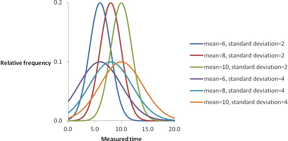
The figure below displays some curves of the normal distribution that plot the relative frequencies of observations against measured times to show how means and standard deviations affect shapes: the means move the curves sideways and the standard deviations affect the height and width of the peaks. The description in terms of relative frequencies and measured times just helps to relate the matter to quality of service measurements; the curves of the normal distribution are widely applicable.
The shape 1/((s/m)*(s/m)) can be found from information about the mean m and the standard deviation s. An estimate of m can be obtained by averaging measured times in the usual way; an estimate of s can be obtained similarly. However, the standard deviation is not determined by the mean though it is estimated from the observations. Both the mean and the standard deviation must be estimated well enough if the relative length of the CI for the mean is to be estimated well enough. This can be done by modifying the formula (z*z)*((s/m)*(s/m))/(r*r) to take account of the uncertainty about the standard deviation: z*z is divided by x*x where x is related to the sample size through the chi squared distribution. For large sample sizes x*x is close to 1, so the earlier formula is recovered.
The formula (z*z)*((s/m)*(s/m))/(r*r), even as modified with x*x, implements a preference for simplicity over accuracy. It underestimates the required sample, and it suggests CIs that are symmetric about the measurement results (though the actual CIs are noticeably asymmetric for some shapes).
The exponential distribution
A distribution of times is sometimes assumed to resemble an exponential distribution: the time that will pass from “now” until the next event occurs is independent of the time that has passed since the previous event. This might apply to events such as call attempts but is unlikely to apply events such as fault reports (as as after a fault report is received, the corresponding repair might be done too late or too hastily to ward off another fault report).
For an exponential distribution, the standard deviation equals the mean. Because of this, the normal distribution of measurements appropriate to the mean can be converted into the normal distribution of measurements appropriate to a q quantile simply by multiplying its standard deviation by √(q/(1-q)). Hence sample sizes and relative lengths of CIs appropriate to the mean can be converted into ones appropriate to quantiles: the relative length of a CI appropriate to the mean is multiplied by √(q/(1-q)) to give the relative length of a CI appropriate to a q quantile with the same sample size. For instance, for an 80 per cent quantile the relative length of a CI appropriate to the mean is multiplied by √(80%/20%), which is 2; thus, for a sample that has mean m and has observation v as the highest among its lowest 80 per cent, if the true value of the mean m is roughly between m*(1-0.1) and m*(1+0.1) then the true value of an 80 per cent quantile is roughly between v*(1-0.1*2) and v*(1+0.1*2).
The gamma distribution
The remarks about quantiles for the exponential distribution illustrates a general point: suppositions about the distribution can refine the definitions of the lengths of the CIs. For this purpose, gamma distributions are useful, as they can model many situations. Here they are used to generalize the exponential distribution in modelling times. In them, for times that are “very” short, shorter measured times occur less frequently than longer ones below a certain time, above which shorter measured times typically occur more frequently than longer ones. This might happen with fault reports if the customers are tolerant, or expect rapid resolution, for a time until they become impatient.
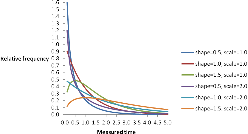
The figure below illustrates gamma distributions for six curves that plot relative frequencies against measured times: each curve shows, in situations represented by that curve, the relative frequencies with which particular measured times occur. If the shape is greater than 1.0 some shorter measured times occur less frequently than some longer ones (so the relative frequency rises from 0.0 to a peak before ultimately falling back towards 0.0); otherwise there are no such times (so the relative frequency consistently falls towards 0.0). If the scale changes the relative frequencies of measured times changes.
In particular, if a curve with shape 1.0 has its scale changed from 1.0 to 2.0, it no longer falls from a relative frequency of 1/1.0 (at a measured time of 0.0) towards a relative frequency of 0.0 but instead falls from a relative frequency of 1/2.0. In addition, if a curve with shape 1.5 has its scale changed from 1.0 to 2.0, it no longer has a peak relative frequency of about 0.48/1.0 (at a measured time of 0.5*1.0) but instead has a peak relative frequency of about 0.48/2.0 (at a measured time of 0.5*2.0).
The best-known gamma distributions have shape 1.0 and scales equal to their means, in which case they are exponential distributions; they fall from their relative frequencies at a measured time of 0.0 towards relative frequencies of 0.0 at “infinity.” Among other important gamma distributions are the chi squared distributions, which have shapes equal to half their “degrees of freedom” and scale 2.0. In particular, a gamma distribution with shape 1.0 and scale 2.0 is also an exponential distribution with mean 2.0 and a chi squared distribution with 2 degrees of freedom.
A simple model of the times taken to set up calls might suppose that the times followed exponential distributions (with different timescales in the two cases). If call set-up always took at least a minimum start time, after which the relative frequencies of times fell away gradually to 0.0, an exponential distribution, displaced to originate at the minimum start time, might still be suitable. However, further investigations might show that call set-up could occur at any time (so the minimum start time was 0.0), often occurred in a range of times higher than that minimum start time, and sometimes occurred at times beyond that range; in such situations, gamma distributions having shapes greater than 1.0 might provide suitable models.
An estimate of the mean time taken, m, can be obtained by averaging measured times in the usual way; an estimate of the standard deviation of the times taken, s, can be obtained similarly. An estimate of the shape of a gamma distribution is 1/((s/m)*(s/m)), and an estimate of the scale is m*((s/m)*(s/m)). Here the ratio s/m is independent of the units in which times are measured. Accordingly, if k Is the shape of the gamma distribution then the sample size is (z*z)*(1/k)/(r*r) where r is independent of the units in which times are measured.
References
ETSI (European Telecommunications Standards Institute). 2019. Speech and Multimedia Transmission Quality (STQ); QoS Aspects for Popular Services in Mobile Networks; Part 6: Post Processing and Statistical Methods. Technical Specification. ETSI TS 102 250-6 V1.3.1 (2019-11). https://www.etsi.org/deliver/etsi_ts/102200_102299/10225006/01.03.01_60/ts_10225006v010301p.pdf.
ITU-T. 2018. Statistical Framework for End-to-End Network Performance Benchmark Scoring and Ranking. ITU-T Recommendation E.840. https://www.itu.int/ITU-T/recommendations/rec.aspx?rec=13621&lang=en.
ITU-T. 2019. Measurement Campaigns, Monitoring Systems and Sampling Methodologies to Monitor the Quality of Service in Mobile Networks. ITU-T Recommendation E.806. https://www.itu.int/ITU-T/recommendations/rec.aspx?id=13924&lang=en.
Last updated on: 19.01.2022